uci is an R package to measure the centrality of cities and regions. The package implements the Urban Centrality Index (UCI) originally proposed by Pereira et al. (2013).

UCI measures the extent to which the spatial organization of a city varies from extreme monocentric to extreme polycentric in a continuous scale, rather than considering a binary classification (either monocentric or polycentric). UCI values range from 0 to 1. Values closer to 0 indicate more polycentric patterns and values closer to 1 indicate a more monocentric urban form.

obs. UCI was originally proposed in the Geographical Analysis Journal. This was my 1st paper (10 years ago!), what makes this a special package to me.

Here’s a simple reproducible example of how it works ( for more info, check the package vignette):

Installation

uci is available on CRAN, so you can install it running:

install.packages('uci')

Data input

The uci package comes with a sample data for demonstration and test purposes. The data is a small sample of the spatial distribution of the population, jobs and schools around the city center of Belo Horizonte, Brazil. This sample data set is a good illustration of the type of data input required by uci.

library(uci)
library(sf)
library(ggplot2)

# load data
data_dir <- system.file("extdata", package = "uci")
grid <- readRDS(file.path(data_dir, "grid_bho.rds"))

head(grid)
#> Simple feature collection with 6 features and 4 fields
#> Geometry type: POLYGON
#> Dimension:     XY
#> Bounding box:  xmin: -43.96438 ymin: -19.97414 xmax: -43.93284 ymax: -19.96717
#> Geodetic CRS:  WGS 84
#>                id population jobs schools                       geometry
#> 1 89a881a5a2bffff        439  180       0 POLYGON ((-43.9431 -19.9741...
#> 2 89a881a5a2fffff        266  134       0 POLYGON ((-43.94612 -19.972...
#> 3 89a881a5a67ffff       1069  143       0 POLYGON ((-43.94001 -19.972...
#> 4 89a881a5a6bffff        245   61       0 POLYGON ((-43.9339 -19.9728...
#> 5 89a881a5a6fffff        298   11       0 POLYGON ((-43.93691 -19.971...
#> 6 89a881a5b03ffff        555 1071       0 POLYGON ((-43.96136 -19.970...

The data is an object of class "sf" "data.frame" with spatial polygons covering our study area and a few columns indicating the number of activities (e.g. jobs, schools, population) in each polygon. Our particular sample data is based on a spatial hexagonal grid (H3 index). While there are advantages of using regular spatial grids to calculate spatial statistics, uci also works with non-regular geometries, such as census tracts, enumeration areas or municipalities.

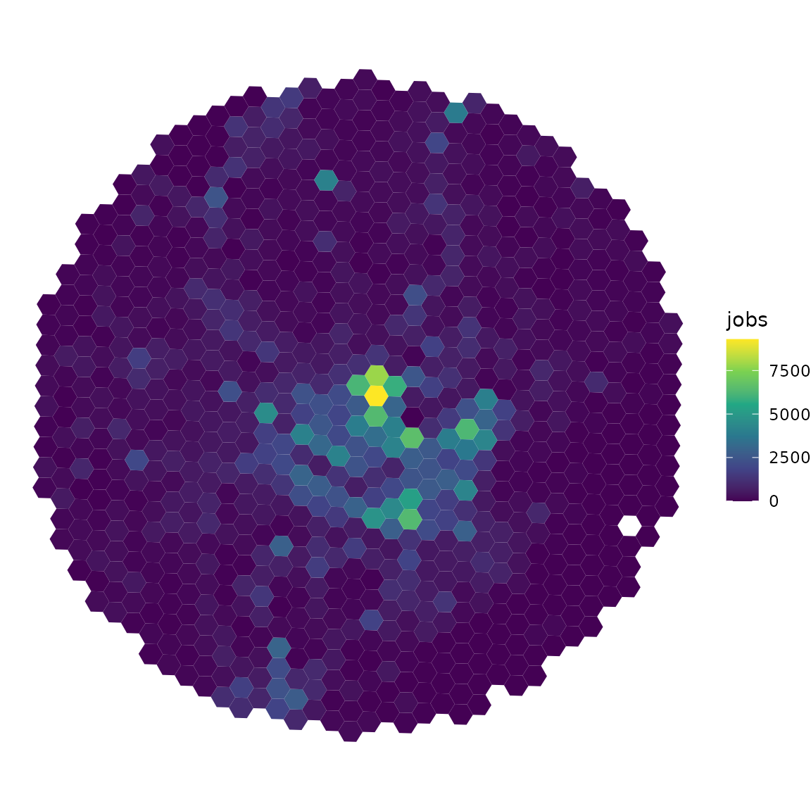
We can visualize the spatial distribution of jobs using ggplot2:

ggplot(data = grid) +
  geom_sf(aes(fill = jobs), color = NA) +
  scale_fill_viridis_c() +
  theme_void()

Calculating UCI

We can easily calculate how mono/polycentric our study area is using the uci()function. In the example below, we consider the spatial distribution of jobs. The output is a data.frame with the value of UCI (0.253) and the components we use to calculate UCI. For more info, check the package vignette.

df <- uci(
  sf_object = grid,
  var_name = 'jobs'
  )

head(df)
#>         UCI location_coef spatial_separation spatial_separation_max
#> 1 0.2538635     0.5278007           3880.114               7475.899