Creating a map of cycling, walking and driving routes in R
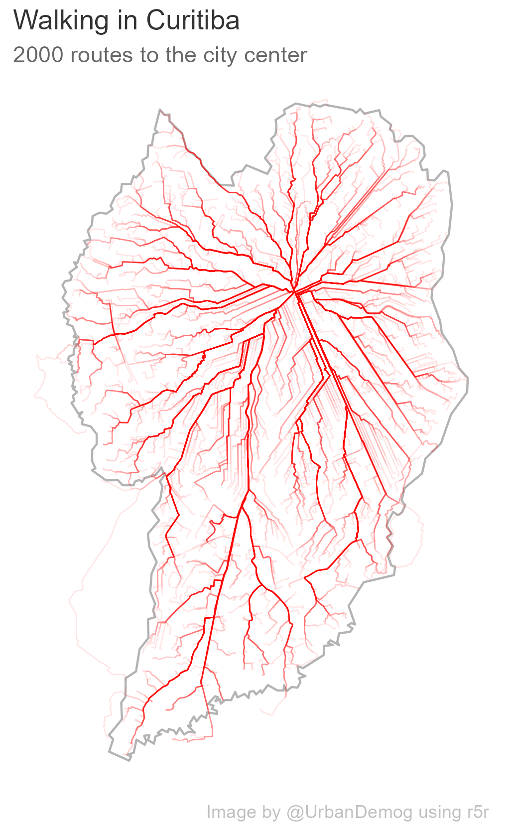
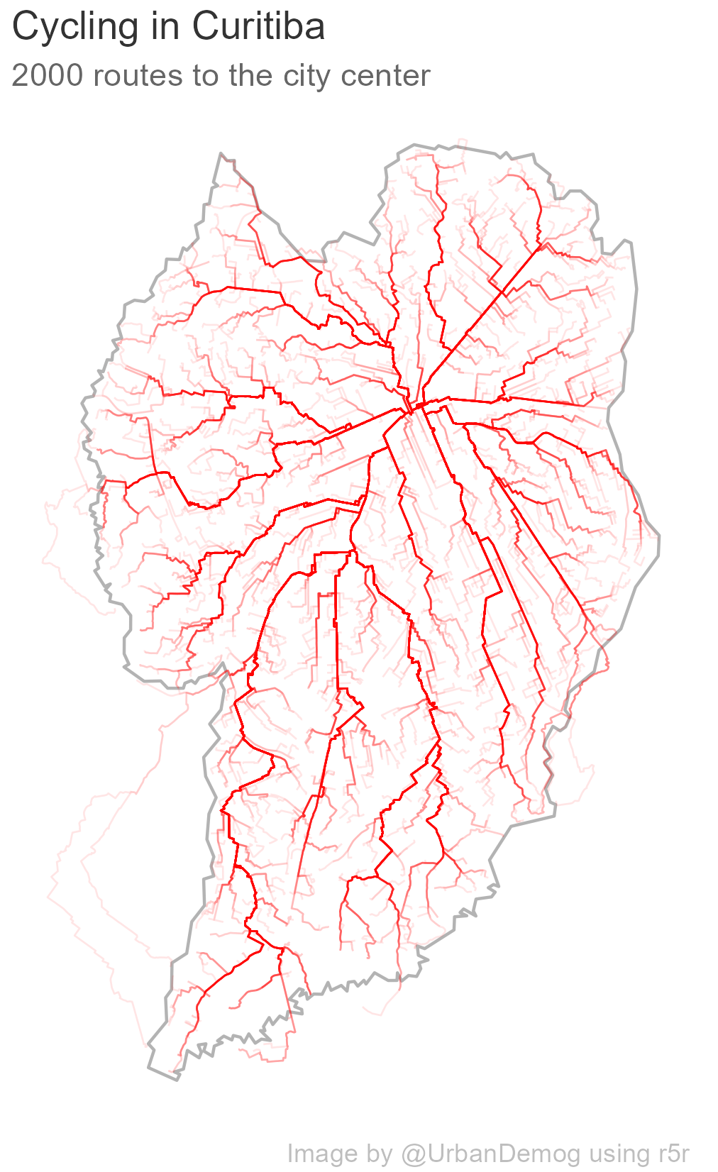
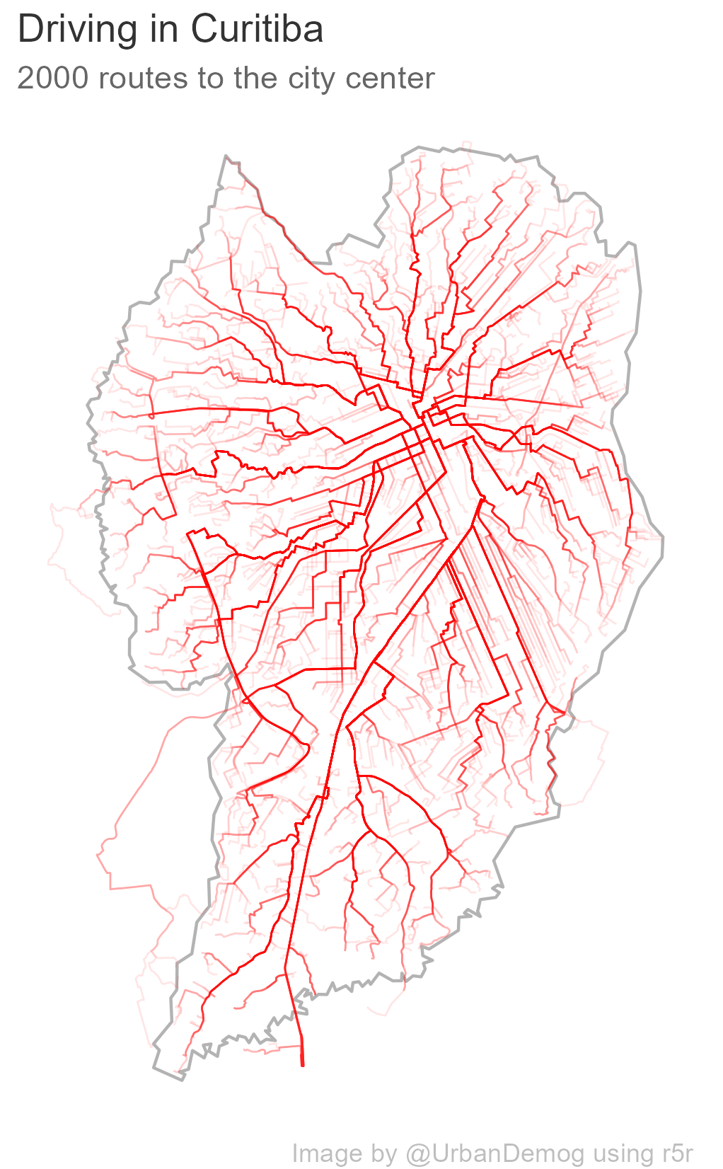
Here’s a quick contribution to the #30DayMapChallenge, day 2 ‘Lines’: a quick reproducible example showing how to use the r5r package to estimate cycling, walking and driving routes in R. In this example, we generate the cycling, walking and driving routes from 2 thousand random locations to the city center in the city of Curitiba, Brazil.
Prepare R environment
options(java.parameters = "-Xmx4G")

library(r5r)
library(geobr)
library(sf)
library(ggplot2)
library(here)
library(osmextract)
library(magrittr)


# create subdirectories "data" and "img"
dir.create(here::here("data"))
dir.create(here::here("img"))
Download the data
# get OSM data
osmextract::oe_download(
  file_url = osmextract::oe_match("Curitiba, Brazil")[[1]],
  download_directory = here::here("data"), force_download = T)

# get city boundaries and city center
city <- 'Curitiba'
city_code <- lookup_muni(name_muni = city)
city_boundary <- read_municipality(code_muni = city_code$code_muni)
city_center <- read_municipal_seat() %>% subset(code_muni == city_code$code_muni)
city_center$id <- 'center'

# get sample of origins in city
set.seed(42)
origins <- st_sample(city_boundary, size = 2000) %>% st_sf()
origins$id <- 1:nrow(origins)

origins <- st_transform(origins, 4326)
city_center <- st_transform(city_center, 4326)
Routing analysis
# build network
r5r_core <- setup_r5(data_path = here::here("data"), verbose = FALSE)

# routing
df <- detailed_itineraries(r5r_core,
                           origins = origins,
                           destinations = city_center,
                           mode = 'bicycle',
                           departure_datetime = as.POSIXct("13-03-2019 14:00:00", format = "%d-%m-%Y %H:%M:%S"),
                           max_trip_duration = 1440,
                           shortest_path = T)
Plot
fig <- ggplot() +
        geom_sf(data = city_boundary, color='gray70', fill=NA) +
        geom_sf(data = df, color='red', alpha=.1, size=.3) +
        labs(title='Cycling in Curitiba',
             subtitle = '2000 routes to the city center',
             caption = 'Image by @UrbanDemog using r5r') +
        theme_void() +
        theme(plot.title = element_text(color = "gray20"),
              plot.subtitle = element_text(color = "gray40"),
              plot.caption = element_text(color = "gray")
              )

# save figure
ggsave(fig, file=here::here("img", "cycling.png"),
       dpi=300, width = 14, height = 14, units = 'cm')