options(java.parameters = "-Xmx4G")

library(r5r)
library(geobr)
library(sf)
library(ggplot2)
library(here)
library(osmextract)
library(data.table)
library(magrittr)


# create subdirectories "data" and "img"
dir.create(here::here("data"))
dir.create(here::here("img"))


# get city boundaries
city <- 'Rio de Janeiro'
city_code <- lookup_muni(name_muni = city)
city_boundary <- read_municipality(code_muni = city_code$code_muni, simplified = F)


# define city center
city_center_df <- data.frame(id='center', lon=-43.182811, lat=-22.906906)
city_center_sf <- sfheaders::sfc_point(obj = city_center_df, x='lon', y='lat')
st_crs(city_center_sf) <- 4326

# define buffer area of analysis 3 Km
buff <- st_buffer(city_center_sf, dist = 3000)

# crs
city_boundary <- st_transform(city_boundary, 4326)
city_center_sf <- st_transform(city_center_sf, 4326)
buff_bb <- st_bbox(buff)


# get OSM data
osmextract::oe_download(provider = 'openstreetmap_fr',
                        file_url = osmextract::oe_match("Rio De Janeiro")[[1]],
                        download_directory = here::here("data"), force_download = T)


# build routing network
r5r_core <- r5r::setup_r5(data_path = here::here("data"), verbose = FALSE)

# get street network as sf
street_network <- r5r::street_network_to_sf(r5r_core)

# drop network outside our buffer
edges_buff <- street_network$edges[buff, ] %>% st_intersection(., buff)
vertices_buff <- street_network$vertices[buff, ] %>% st_intersection(., buff)
city_boundary_buff <- st_intersection(city_boundary, buff)
plot(city_boundary_buff)

# add id to vertices
vertices_buff$id <- vertices_buff$index


# calculate travel times to city center 
tt <- r5r::travel_time_matrix(r5r_core,
                              origins = vertices_buff,
                              destinations = city_center_df,
                              mode = 'walk')


# add travel time info to street network
tt$fromId <- as.numeric(tt$fromId)
setDT(edges_buff)[tt, on=c('from_vertex'='fromId'), travel_time := i.travel_time]
edges_buff <- st_sf(edges_buff)

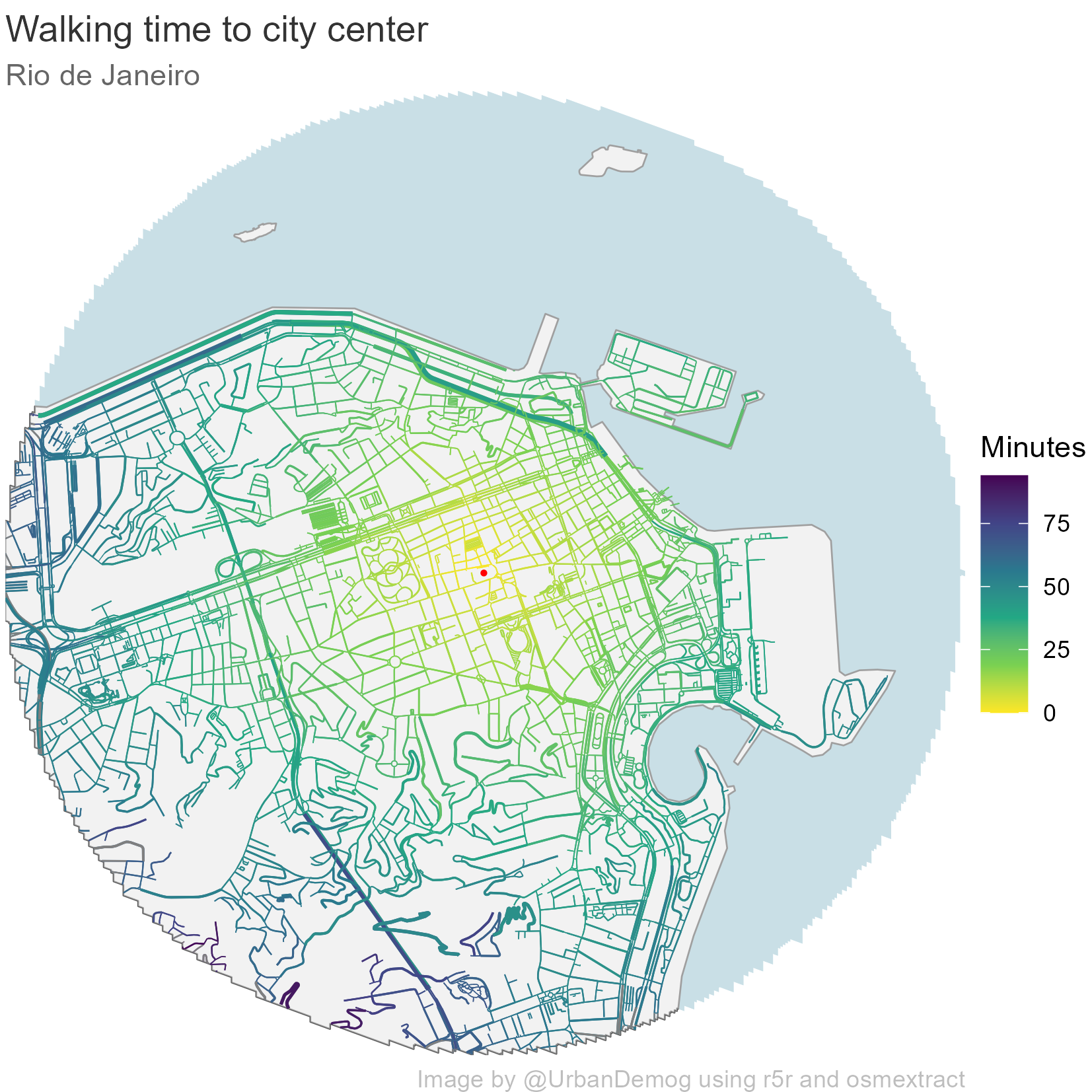
Now we only need to plot and save the figure.

# figure
temp <- ggplot() + 
        geom_sf(data=buff, fill='lightblue', color=NA)  +
        geom_sf(data=city_boundary_buff, fill='white', size=.3)  +
        geom_sf(data=buff, fill='gray90', color=NA, alpha=.5)  +
        geom_sf(data=edges_buff, aes(color=travel_time, size=length))  +
        geom_sf(data=city_center_sf, color='red', size=.5) +
        scale_size_continuous(range = c(0.1, .8), guide='none') +
        scale_color_viridis_c(direction = -1) +
  labs(title='Walking time to city center',
       subtitle = 'Rio de Janeiro',
       caption = 'Image by @UrbanDemog using r5r and osmextract',
       color='Minutes') +
  coord_sf(xlim = c(buff_bb[[1]], buff_bb[[3]]), 
                 ylim = c(buff_bb[[2]], buff_bb[[4]]), expand = FALSE) + 
  theme_void() +
  theme(plot.background = element_rect(fill = "white", color='white'),
        plot.title = element_text(color = "gray20"),
        plot.subtitle = element_text(color = "gray40"),
        plot.caption = element_text(color = "gray"))
        
# save figure
ggsave(temp, file=here::here("img", "aa32k.png"), 
       dpi=300, width = 14, height = 14, units = 'cm')